
Because it is sometimes difficult to find the right product in our long list of products, we aim to advise you as much as possible. This can be in the form of theoretical knowledge of certain properties, or a simple comparison between the pros and cons of products. This article helps to explain the former; the theoretical knowledge of certain properties. It is intended as a guide and to explain the various properties mentioned in the data sheets of the oscilloscopes.
The data sheets of most explain much more than just the number of channels or the bandwidth of a scope. This article provides an overview of the common terms in the data sheet of a scope. If a unit is available for the specification, it is indicated in square brackets.
Content
- Amplitude
- Bandwidth
- Connectivity
- Division
- Fourier transform
- Memory
- Holdoff range
- Interpolation
- Channels
- Math operations
- Rise time
- Sample Rate
- Triggers
- Vertical sensitivity
- Vertical resolution
- Waveform capture rate
Amplitude

Alternative concept use for amplitude
Amplitude, as a general technical term, is defined as the maximum deviation from zero or "equilibrium". Thus, when a sine wave is measured with an oscilloscope, amplitude will be the amplitude of the sine wave.
Some oscilloscope brands use a different definition for understanding amplitude. An example of this can be seen next to this where, in this case for Siglent, the amplitude is shown as the difference between the most likely "higher state" (top) and most likely "lower state" (base). These different definitions can always be found in the manual of the relevant product.
Bandwidth (bandwidth) [Hz]

The -3dB point.
The bandwidth is probably the most important feature of any scope because it describes up to which frequency signals can be measured. This determines the fundamental ability to measure signals. The scope can display the signals accurately and faithfully up to this value. The bandwidth is specified as the frequency at which the -3dB point is reached. This is the frequency point at which a measured sinusoid is attenuated until it is measured at 70.7% of the original signal strength. Without a solid bandwidth, the other features of your scope will not be very useful and details will get lost, turning various calculations relatively pointless. To be sure of the sufficient bandwidth, it is best to use a simple calculation: Bandwidth ≥ Highest frequency component of the signal x 5.

Example of connectivity.
Connectivity
This specification is completely preferential as some scopes can be connected to numerous devices, while other scopes only have a trigger output. The requirements depend on what it will be used for. Will the scope often be operated via a computer, or will the data be used for comparison purposes with simulation values? Then a USB host or device connection is definitely useful. Connectivity is not necessary if the scope only needs to display the signals and not analyse them. Most scopes offer some connectivity by default.
EthernetA LAN connector offers the possibility to connect the scope to a computer, allowing the scope to be managed via the network. This offers extensive possibilities that are very useful in a lab, for example.
GPIB / RS-232These connections offer parallel communication possibilities with a computer or other device and are less common on scopes.
Pass/Fail outputThis output is key when testing multiple products. If a certain requirement has been set up which the output needs to meet, automatic batch testing can be done via the pass/fail output. This is especially useful in a professional environment.
TriggerA trigger connector can trigger the scope through another device, for example a function generator. This provides a stable triggering that can lead to the ability to measure signals that are not suitable to trigger individually. Noise is a good example of this.
VGASome scopes provide image outputs that allow a direct connection to a monitor.
USBA USB connection comes in two forms, called host and device. These two types describe how the communication works and whether the device can be connected directly to a computer. A USB host connection can write data on storage devices, for example on a memory stick. Measurements can be displayed directly on a computer when you connect the scope to a USB device. A division on a scope screen. A division is one box on an oscilloscope screen.
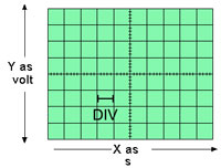 One division is one box on an oscilloscope's screen. DivisionA box on the screen of the scope. Many settings are related to this, for example the vertical and horizontal settings. Almost all scopes use the settings per division. This makes it easy to see how much amplitude a signal has. FFT at changing signal. Example of an FFT calculation on a frequency changing signal. |
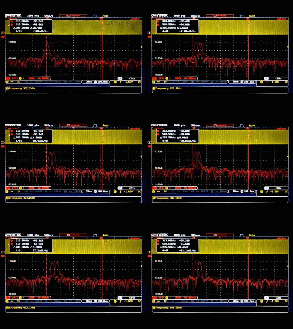 Example of an FFT calculation on a frequency changing signal. Fourier transformation (FFT)FFT enables the scope to indicate which frequencies are present in the signal and how strong these components are. The FFT is a useful tool when analysing FM signals, for example, as they always have at least 2 frequency components that are not easy to find in the time domain. Different scopes offer different experiences, which are not always clearly explained in the specifications. |
Memory depth [points] of [pts]
This number describes the memory size of a scope, i.e. how many points can be stored per measurement of the signal. The higher the value, the more details can be showed in the signal display. A high memory depth can display the same measurement time in more detail, if the sample rate is sufficient.
Holdoff range [s]
This specification is related to the triggering and describes how long the scope will wait before it looks for a new trigger point.
Interpolation

Comparison of the two interpolation methods
There are two main types of interpolation: sin x/x and linear. Both types are often supported by scopes. Sin x/x connects the sampled values to a curved line, while linear forms straight lines. Both interpolation methods have their advantages. Sin x/x, for example, offers better results with sinusoidal signals, while linear signals do better with square or sawtooth signals. The interpolation method also influences the sampling rate.
A sinusoidal signal can accurately represent an interpolation method with sin x/x if the sampling rate is 2.5 times higher than the frequency of the signal. Whereas with linear interpolation no good representation can be given if this is a factor of 10.

Typical appearance of the connectors of a scope.
Channels
The more channels a scope has, the more different signals can be displayed simultaneously. It is important to keep an eye on the sample rate for this specification. Often the sample rate is distributed among the channels and resolution can get lost when multiple channels are connected.
Math operations
A scope can often not only display signals, but also perform calculations on the signals such as adding or multiplying two signals. In addition, many scopes also offer the possibility to perform a Fast Fourier Transform (FFT) on the signal. The extent of the number of operations that can be performed is often very diverse, ranging from only basic functions to highly complicated functions that the users can enter themselves.

The definition of rise time.
Rise time [s]
The rise time is key when measuring digital signals. This describes the time the scope needs to follow a pulse. More specifically, it is the time it takes for the scope to increase from 10 - 90% of the signal strength. When following a digital 0 to 1 switch-over, signal details will be lost in the time needed to go from low to high. The lower the rise time, the higher the detail of the signal. The rise time is almost always inversely proportional to the bandwidth, i.e., a higher bandwidth requires a lower rise time.
Sample rate [Sa/s]

The effect of a higher sample rate.
The sample rate describes how often the input values are looked at during 1 second. This is measured in samples per second. Generally speaking, the higher the better for this value. A scope with a high sample rate can measure and display signals in more detail. Critical information will be lost less frequently during the acquisition thanks to this feature. The desired sample rate depends on the type of interpolation that the scope uses. At sin(x)/x interpolation, the minimum sample rate needs to be about 2.5 times as high as the highest frequency in the signal, while at linear interpolation it needs to be about 10 times as high for an accurate reconstruction.
Triggers
The trigger possibilities of a scope are critical for a stable view of the signal. There are a number of different trigger methods that can all be used in different ways to ensure that the signal is clearly displayed. An example of a triggering is "Rising-edge" which looks at when a signal surpasses a certain adjustable threshold value. This allows, for example, square waves and sinusoids to be displayed easily.
Vertical sensitivity [V]
This property describes the smallest peak values that the scope can measure and boost. Most scopes range from 1 or 10 mV to 10 V per division, so both tiny and big signals can be displayed.
Vertical resolution [bit]

The effect of a higher number of bits.
This number describes how many binary numbers a scope has in order to display different voltages in the signal. This number is related to the Analogue-Digital converter, or AD-converter (ADC). Many scopes have an 8-bit ADC, which allows about 256 levels to be measured between the minimum and maximum values. This applies on any scale, so from the 1 mV to 10 V/division. Certain calculation methods can improve the resolution afterwards.
Waveform capture rate [wfm/s]
This specification explains the ability of the scope to learn properties of a signal. This also depends on the sample rate, but there is a big difference between what these specifications demonstrate exactly. All scopes have a so-called 'dead-time' between each measurement. During this time, the scope processes the obtained signal and performs calculations. The scope will not register what is going on with the input during the dead-time. If something happens to the signal during this time, the scope will not register it and will not display it on the screen. A higher wfm/s means that there is a smaller chance that signal properties will be missed because the dead-time is smaller. Some scopes offer a "burst mode". This mode offers an extremely high capture speed for a certain amount of time after which in a longer consecutive period of time all processing is done, resulting in longer blocks during the dead-time.





